大家好,我是小小明。
前面我已经用Python求积分解决了一道小学数学题,详见:Python神器可以拯救小学数学题不会做
结果今天又碰到一道更难的,题目如下:

今天我们将尝试尽量多的通过Python来解题。
首先我们以左下角为原点建立直角坐标系,很快能够知道圆的方程为 ( x − 5 ) 2 + ( y − 5 ) 2 = 5 2 (x-5)^2+(y-5)^2=5^2 (x−5)2+(y−5)2=52
两个扇形的方程分别为 ( x − 10 ) 2 + y 2 = 1 0 2 (x-10)^2+y^2=10^2 (x−10)2+y2=102和 x 2 + ( y − 10 ) 2 = 1 0 2 x^2+(y-10)^2=10^2 x2+(y−10)2=102的一部分。
上面的方程很容易得到,但要计算出方程表达式还需费一番功夫,所以下面我们打算也让Python来计算。
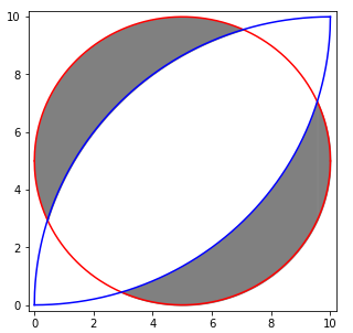
在解题前,我们会先用Python绘制出如下图像:
绘图步骤
画圆
首先计算出上半圆和下半的表达式分别为:
from sympy.abc import x, y
import sympy

c1, c2 = sympy.solve((x-5)**2+(y-5)**2 - 5**2, y)
display(c1)
display(c2)
结果:
5 − − x ( x − 10 ) \displaystyle 5 - \sqrt{- x \left(x - 10\right)} 5−−x(x−10)
x ( 10 − x ) + 5 \displaystyle \sqrt{x \left(10 - x\right)} + 5 x(10−x)+5
如果想要展开表达式可以进行如下操作:
display(sympy.expand(c1))
display(sympy.expand(c2))
结果:
5 − − x 2 + 10 x \displaystyle 5 - \sqrt{- x^{2} + 10 x} 5−−x2+10x
− x 2 + 10 x + 5 \displaystyle \sqrt{- x^{2} + 10 x} + 5 −x2+10x+5
直接打印可以看到在Python的表达式:
print(str(c1))
print(str(c2))
5 - sqrt(-x*(x - 10))
sqrt(x*(10 - x)) + 5
因此利用上述文本,我们可以直接进行numpy的函数求值,下面尝试画个圆试一下:
import numpy as np
from numpy import sqrt
import matplotlib.pyplot as plt

%matplotlib inline

plt.figure(figsize=(5, 5))
x = np.linspace(0, 10, 1024)

plt.plot(x, eval(str(c1)), color="r")
plt.plot(x, eval(str(c2)), color="r")

plt.xlim(-0.2, 10.2)
plt.ylim(-0.2, 10.2)

plt.show()
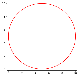
可以看到我们求解的两个表达式可以画出圆形。
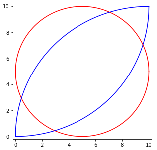
下面我们继续来画扇形:
画扇形
两个扇形的方程分别为 ( x − 10 ) 2 + y 2 = 1 0 2 (x-10)^2+y^2=10^2 (x−10)2+y2=102和 x 2 + ( y − 10 ) 2 = 1 0 2 x^2+(y-10)^2=10^2 x2+(y−10)2=102的一部分。
首先我们计算上面的扇形的函数公式:
sympy.solve((x-10)**2+y**2 - 10**2, y)
结果:
[sqrt(x*(20 - x)), -sqrt(-x*(x - 20))]
显然上面的扇形的函数公式是正数,可以直接取角标为0的函数公式:
s1, _ = sympy.solve((x-10)**2+y**2 - 10**2, y)
s1
结果:
x ( 20 − x ) \displaystyle \sqrt{x \left(20 - x\right)} x(20−x)
用同样的方法我们再求出下面的扇形:
s2, _ = sympy.solve(x**2+(y-10)**2 - 10**2, y)
s2
结果:
10 − 100 − x 2 \displaystyle 10 - \sqrt{100 - x^{2}} 10−100−x2
然后我们绘制函数图形验证一下:
import numpy as np
from numpy import sqrt
import matplotlib.pyplot as plt
from sympy.abc import x, y
import sympy

%matplotlib inline

c1, c2 = sympy.solve((x-5)**2+(y-5)**2 - 5**2, y)
s1, _ = sympy.solve((x-10)**2+y**2 - 10**2, y)
s2, _ = sympy.solve(x**2+(y-10)**2 - 10**2, y)

x = np.linspace(0, 10, 1024)

plt.figure(figsize=(5, 5))
plt.plot(x, eval(str(c1)), color="r")
plt.plot(x, eval(str(c2)), color="r")

plt.plot(x, eval(str(s1)), color="b")
plt.plot(x, eval(str(s2)), color="b")

plt.xlim(-0.2, 10.2)
plt.ylim(-0.2, 10.2)

plt.show()
绘制阴影
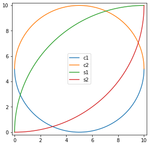
首先我们需要求出四个交点。
先分清几个线各是哪条:
import numpy as np
from numpy import sqrt
import matplotlib.pyplot as plt
from sympy.abc import x, y
import sympy

%matplotlib inline

c1, c2 = sympy.solve((x-5)**2+(y-5)**2 - 5**2, y)
s1, _ = sympy.solve((x-10)**2+y**2 - 10**2, y)
s2, _ = sympy.solve(x**2+(y-10)**2 - 10**2, y)

x = np.linspace(0, 10, 1024)

plt.figure(figsize=(5, 5))
plt.plot(x, eval(str(c1)), label="c1")
plt.plot(x, eval(str(c2)), label="c2")

plt.plot(x, eval(str(s1)), label="s1")
plt.plot(x, eval(str(s2)), label="s2")

plt.xlim(-0.2, 10.2)
plt.ylim(-0.2, 10.2)
plt.legend()

plt.show()
下面分别交出交点:
from sympy.abc import x, y

x1, = sympy.solve(c1-s1, x)
x2, = sympy.solve(c1-s2, x)
x3, = sympy.solve(c2-s1, x)
x4, = sympy.solve(c2-s2, x)
x1, x2, x3, x4
(15/4 - 5*sqrt(7)/4,
 25/4 - 5*sqrt(7)/4,
 5*sqrt(7)/4 + 15/4,
 5*sqrt(7)/4 + 25/4)
根据对称性,我们可以知道四个交点的坐标分别为(x1,x2), (x2,x1), (x3,x4),(x4,x3)
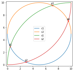
同样可以画图验证一下:
import numpy as np
from numpy import sqrt
import matplotlib.pyplot as plt
from sympy.abc import x, y
import sympy

%matplotlib inline

c1, c2 = sympy.solve((x-5)**2+(y-5)**2 - 5**2, y)
s1, _ = sympy.solve((x-10)**2+y**2 - 10**2, y)
s2, _ = sympy.solve(x**2+(y-10)**2 - 10**2, y)
x1, = sympy.solve(c1-s1, x)
x2, = sympy.solve(c1-s2, x)
x3, = sympy.solve(c2-s1, x)
x4, = sympy.solve(c2-s2, x)

x = np.linspace(0, 10, 1024)

plt.figure(figsize=(5, 5))
plt.plot(x, eval(str(c1)), label="c1")
plt.plot(x, eval(str(c2)), label="c2")

plt.plot(x, eval(str(s1)), label="s1")
plt.plot(x, eval(str(s2)), label="s2")

plt.plot([x1, x2, x3, x4], [x2, x1, x4, x3], 'rx')
plt.text(x1, x2+0.1, "p1", ha="center", va="bottom")
plt.text(x2, x1+0.1, "p2", ha="center", va="bottom")
plt.text(x3, x4+0.1, "p3", ha="center", va="bottom")
plt.text(x4, x3+0.1, "p4", ha="center", va="bottom")

plt.xlim(-0.2, 10.2)
plt.ylim(-0.2, 10.2)
plt.legend()
plt.show()
下面开始绘制阴影:
import numpy as np
from numpy import sqrt
import matplotlib.pyplot as plt
from sympy.abc import x, y
import sympy

%matplotlib inline

c1, c2 = sympy.solve((x-5)**2+(y-5)**2 - 5**2, y)
s1, _ = sympy.solve((x-10)**2+y**2 - 10**2, y)
s2, _ = sympy.solve(x**2+(y-10)**2 - 10**2, y)
x1 = sympy.solve(c1-s1, x)[0].evalf()
x2 = sympy.solve(c1-s2, x)[0].evalf()
x3 = sympy.solve(c2-s1, x)[0].evalf()
x4 = sympy.solve(c2-s2, x)[0].evalf()


x = np.linspace(0, 10, 1024)
c1, c2, s1, s2 = map(lambda s: eval(str(s)), (c1, c2, s1, s2))

plt.figure(figsize=(5, 5))
plt.plot(x, c1, label="c1")
plt.plot(x, c2, label="c2")
plt.plot(x, s1, label="s1")
plt.plot(x, s2, label="s2")

plt.fill_between(x[x <= x1], c1[x <= x1], c2[x <= x1], color="grey")
plt.fill_between(x[(x1 < x) & (x <= x3)], s1[(x1 < x) &
                 (x <= x3)], c2[(x1 < x) & (x <= x3)], color="grey")
plt.fill_between(x[(x2 <= x) & (x <= x4)], c1[(x2 <= x) & (
    x <= x4)], s2[(x2 <= x) & (x <= x4)], color="grey")
plt.fill_between(x[x > x4], c1[x > x4], c2[x > x4], color="grey")

plt.plot([x1, x2, x3, x4], [x2, x1, x4, x3], 'rx')

plt.xlim(-0.2, 10.2)
plt.ylim(-0.2, 10.2)
plt.legend()
plt.show()
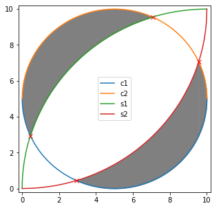
然后再稍微调整一下颜色即可得到文章开头的图像:
绘图完整代码
import numpy as np
from numpy import sqrt
import matplotlib.pyplot as plt
from sympy.abc import x, y
import sympy

%matplotlib inline

c1, c2 = sympy.solve((x-5)**2+(y-5)**2 - 5**2, y)
s1, _ = sympy.solve((x-10)**2+y**2 - 10**2, y)
s2, _ = sympy.solve(x**2+(y-10)**2 - 10**2, y)
x1 = sympy.solve(c1-s1, x)[0].evalf()
x2 = sympy.solve(c1-s2, x)[0].evalf()
x3 = sympy.solve(c2-s1, x)[0].evalf()
x4 = sympy.solve(c2-s2, x)[0].evalf()


x = np.linspace(0, 10, 1024)
c1, c2, s1, s2 = map(lambda s: eval(str(s)), (c1, c2, s1, s2))

plt.figure(figsize=(5, 5))
plt.plot(x, c1, label="c1", color="r")
plt.plot(x, c2, label="c2", color="r")
plt.plot(x, s1, label="s1", color="b")
plt.plot(x, s2, label="s2", color="b")

plt.fill_between(x[x <= x1], c1[x <= x1], c2[x <= x1], color="grey")
plt.fill_between(x[(x1 < x) & (x <= x3)], s1[(x1 < x) &
                 (x <= x3)], c2[(x1 < x) & (x <= x3)], color="grey")
plt.fill_between(x[(x2 <= x) & (x <= x4)], c1[(x2 <= x) & (
    x <= x4)], s2[(x2 <= x) & (x <= x4)], color="grey")
plt.fill_between(x[x > x4], c1[x > x4], c2[x > x4], color="grey")

plt.xlim(-0.2, 10.2)
plt.ylim(-0.2, 10.2)
plt.show()
在完成图像绘制后,我们就可以通过相同的思路求积分得到面积了:
积分求解面积
最终结果完整求解代码:
from sympy.abc import x, y
from sympy import integrate
import sympy

c1, c2 = sympy.solve((x-5)**2+(y-5)**2 - 5**2, y)
s1, _ = sympy.solve((x-10)**2+y**2 - 10**2, y)
s2, _ = sympy.solve(x**2+(y-10)**2 - 10**2, y)
x1 = sympy.solve(c1-s1, x)[0].evalf()
x2 = sympy.solve(c1-s2, x)[0].evalf()
x3 = sympy.solve(c2-s1, x)[0].evalf()
x4 = sympy.solve(c2-s2, x)[0].evalf()

r = integrate(c2-c1, (x, 0, x1))+integrate(c2-s1, (x, x1, x3)) + \
    integrate(s2-c1, (x, x2, x4))+integrate(c2-c1, (x, x4, 10))
r.round(8)
结果:29.27625191
如果希望得到更加精确的的结果,可以最后再调用evalf方法:
from sympy.abc import x, y
from sympy import integrate
import sympy

c1, c2 = sympy.solve((x-5)**2+(y-5)**2 - 5**2, y)
s1, _ = sympy.solve((x-10)**2+y**2 - 10**2, y)
s2, _ = sympy.solve(x**2+(y-10)**2 - 10**2, y)
x1, = sympy.solve(c1-s1, x)
x2, = sympy.solve(c1-s2, x)
x3, = sympy.solve(c2-s1, x)
x4, = sympy.solve(c2-s2, x)

r = integrate(c2-c1, (x, 0, x1))+integrate(c2-s1, (x, x1, x3)) + \
    integrate(s2-c1, (x, x2, x4))+integrate(c2-c1, (x, x4, 10))
r.evalf()
结果:29.2762519060696